Mandelbrot-256
Fractals, Basic-256 and BTK2
Introduction
What is it?
Mandelbrot-256 is a small demo program that will allow you not just to display but also to
explore the Mandelbrot set. It is written in Basic-256 and it uses the BTK2 GUI toolkit routines. It allows one to :
-/ draw the Mandelbrot fractal (obviously..)
-/ explore and render Julia sets (With a nice & fast preview)
-/ look at the orbits of the complex coordinates as they are being calculated
-/ zoom into the Mandelbrot set (The fun part of the program!)
-/ adapt the color scheme to be used (not all that stable code though.)
Why create
it?
The BTK2 GUI Toolkit is a set of subroutines I wrote to handle the drudgery of drawing normal buttons, radio-buttons, tabs, sliders, etc on the graphical output screen (of course, quite some coding is still required to use these in a real-world scenario.) Simple example programs for each of these elements can be found on the demo page.
My main aim with Mandelbrot-256 was not to write a real fractal/Mandelbrot program, but to use this popular subject in order to write a program that would show that the BTK-256 routines could be used to make relatively good looking, full-featured programs.
(Of course, BTK2 can also providing some GUI eye-candy to the simple, one-off Basic-256 programs of the style to be found in the examples directory.)
You will be the judge of whether I was successful or not.
How do I use
the program?
Of course, beyond a certain complexity, a program needs a user guide on how to use it. (We cannot all be Apple software Engineers.) This document aims to explain the main functionalities of the program. Of course, being Basic-256, the code is visible to all for analysis and can be improved by anyone interested to try.
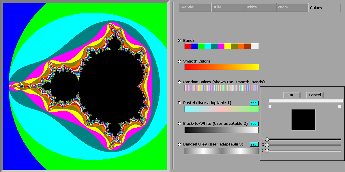
The Main screens
Splash
screen
When you start the program, you are presented with a pretty bare-bones Splash screen
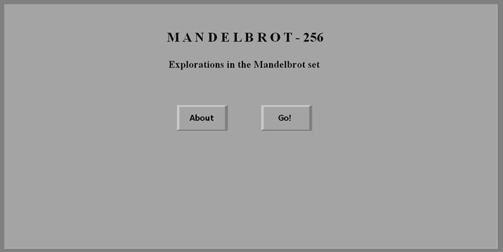
A basic, grey affair, the Splash screen sports an About- and a Go!-button. The functionality of these two is rather obvious so needs no explanation.
A small particle system has been embedded to provide some useless animation when the Go! Is pressed.
Default start-up view
When leaving the Splash screen, the start-up view is presented, showing the general setup of the main program:
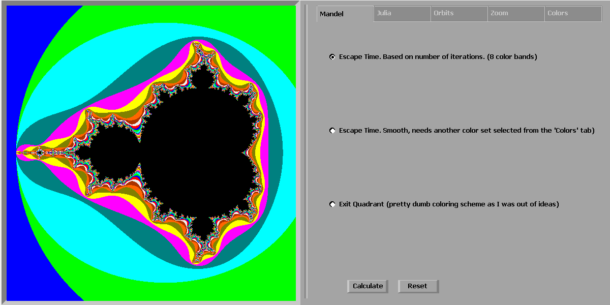
The GUI is split in two parts: a main graphical output area on the left, currently showing a Mandelbrot set and a tabbed configuration/preview area on the right, currently showing the options belonging to the Mandel-tab.
Mandel-tab
The Mandel-tab area has 3 radio-buttons, each selecting a different algorithm to color the outside of the Mandelbrot set (the colors to be used are located under the Colors-tab). The default coloring algorithm (so the one used at startup) is Escape Time (banded)
Escape Time (banded)
Here, the coloring is simply based on the number of iteration it takes before the coordinate reaches an escape value. The corresponding default color-bar consists of nine contrasting colors. The stepwise increase in number of iterations means that large area bands have the same escape value and hence the same color. This can be very useful for showing the structure at deeper zoom levels. (examples later)
This algorithm, which by default uses a banded color-bar (see Colors-tab), can use any other 256-slot color-bar as well. It will just ignore the gradation and select the color based in jumps of 30 slots. This is the default and is the same as the above picture
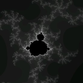
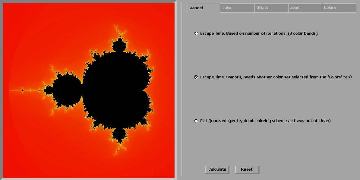
Escape Time (smooth)
The coloring here is smoothed by renormalizing the iteration count. This way, one can obtain a fractional transition between two escape iterations by measuring how far the iterated point landed outside of the escape cutoff
This algorithm will refuse to use the banded color-bar (since by definition it will not be smooth) and, when forced to use it anyway, will pop up a message indicating that another color-bar needs to be used. So, to use smooth, first go select another color-bar in the Colors-tab, then come back to Mandel-tab, select EscapeTime (smooth) and click the Calculate button.
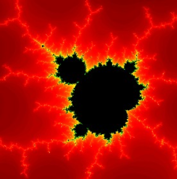
The difference between banded and smooth can best be seen by selecting the multi-colored User 2 color-bar. banded will show large areas with the same color (representing the number of iterations needed to escape), especially at the furthest distances outside the set, while smooth will show a lot more bands in the same areas (representing the distance from the escape value at escape).
To show the difference between smooth and banded, here are two renders using the User2 color-bar. One can see that there are a lot more bands in the smooth algorithm, leading to, euh, smoother results when using a nice color transition like the one above.

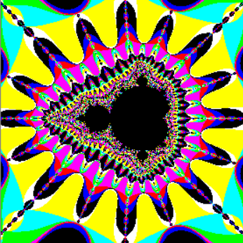
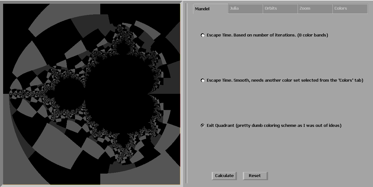
Exit Quadrant
The third coloring scheme is there a bit as a filler.
It is a very simple coloring scheme is based on the complex quadrant from which the point escapes
So, if after x iterations the resulting complex coordinate is deemed to have escaped, we look in which quadrant this escaped coordinate lies and base the color on this.
The actual colors chosen are also based on the color-bar selected in the Colors-tab. None of the color-bars however give a nice contrasting set of colors though.
The Mandel-tab area also has 2 action-buttons, Calculate and Reset
Calculate will redo the Mandelbrot calculation using the selected coloring algorithm in combination with the chosen color-bar for the previously selected coordinates.
Reset can be used to completely reset the program. This means that the default Escape Time (banded) will be selected in combination with the default, contrasting color-bar to re-render the Mandelbrot set according to the default coordinates, leaving you with the same screen the program started with (minus the splash-screen)
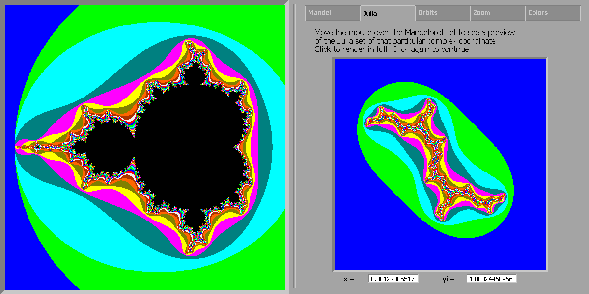
The Julia-tab area is rather sparse. It just has 2 text-boxes, some explanatory text and a preview window. The moment you move over the Mandelbrot set, the preview window will show you an outline of the Julia set for that particular coordinate.
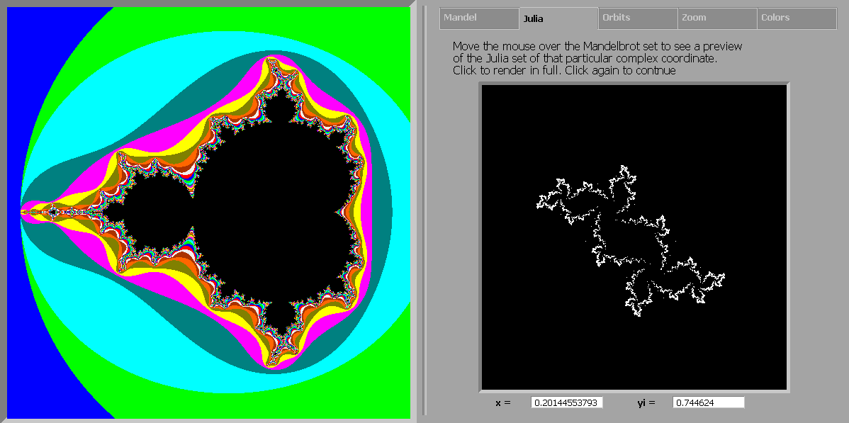
Julia uses the location of the mouse (when the mouse
position is over the main graphical output area) to show the complex coordinates of the mouse location in the 2
textboxes and will generate, on the fly, an outline of the Julia set in the
preview window corresponding to the coordinates the mouse is pointing to.
This real-time algorithm to create the Julia-set preview is called the Inverse Iteration Method (IIM)
Clicking the left mouse button in this mode (so while the mouse is over the Mandelbrot area) will show a fully rendered Julia set of that particular point in the preview window, using the selected coloring algorithm from the Mandel-tab and the selected color-bar from the Colors-tab.
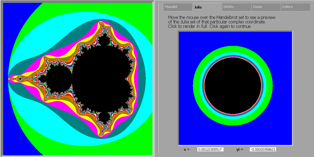
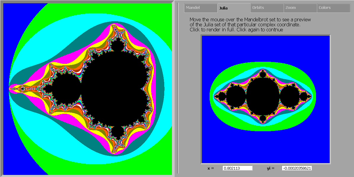
Here are some examples:
(0,0) will show you the unit circle. Of course, this is about the least interesting Julia set of them all.
(0.8,0) will show you the San Marco Julia set which resembles the San Marco in Venice, mirrored in the lagoon. (ok, with a lot of imagination)
(0,1) is one of my favorites and show a lightning-like construction
Orbits-tab
The Orbits-tab uses the same layout as the Julia-tab ie 2 text fields for the complex coordinates, some instructions on how to use it, and a huge graphical output window for the orbit calculation.
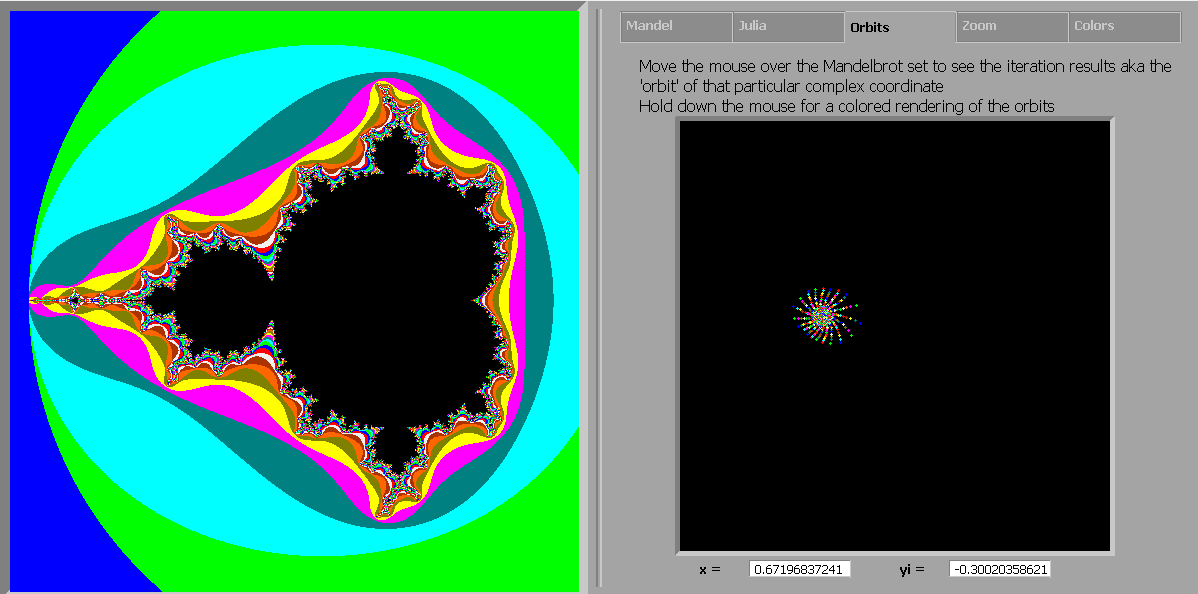
The idea behind the Orbits-tab is to show the evolution of
the coordinate under the mouse pointer after every iteration. When the point escapes (as
happens in the colored areas), the output area is cleared and the calculation
restarted (this causes a slight flickering of the output area).
If the point belongs to the set, the calculation continues indefinitely while the points are
pulled to their basin of attraction. (hence no flicker.) The newly calculated
point is drawn in white while the previously calculated point is drawn in grey.
As shown in the text in the initial output area, holding the left mouse down while moving over the Mandelbrot set will show the orbit evolutions of the different points superimposed on each other. Each new orbit calculation will have a new color, again based on the selected color-bar.
What is so interesting about visualizing the orbit evolution? you might ask. Well, it shows a bit the deeper structure of the Mandelbot set.
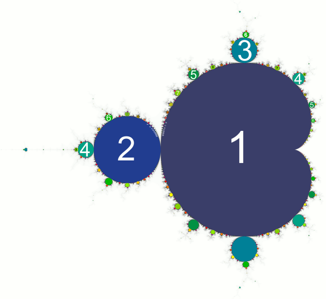
When looking at the Mandelbrot set, you immediately see the
large cardioid-shaped region in the center (The big circle with the dent on the
right). This cardioid is the
region where the iterations result in a single attracting fixed point. The
Orbits-tab will show a lot of shapes (point, lines, start, spirals, etc)
in this area but all shapes end up in a fixed point. This can best be seen in a point
like (-0.268575,0.473119) where you see the spiral arms contracting to a single point.
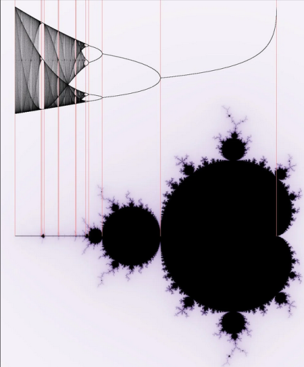
To the left of the main cardioid, is a circular-shaped bulb. In this bulb, the iterations result in an attracting cycle of period 2 ie two points. (in fact, the line along the axis from right to left corresponds nicely to the bifurcation diagram. You can even find the period 3 attractor around (1.75,0):
Orbits can show that all the bulbs around the main cardioid
correspond to specific attracting cycles. The top one corresponds to cycle 3.
The next biggest one (at about 45 degrees) is cycle 4, then 5, then 6 etc. You can
find nice looking orbit evolutions in the border areas between the main
cardioids and these bulbs, especially in zoomed mode. Orbits, due to their dynamic nature, really do not come into
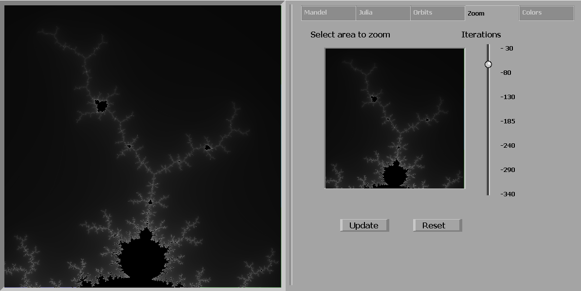
their own in screenshots.. Zoom-tab This is where the most fun is to be had. The Zoom-tab shows a mini-version of the graphical output
window. You can rectangle-select an area in this mini-version corresponding to
where you want to zoom into. (the rectangle select code is rather primitive and
does not visually allow you to make the selected area smaller) The program
will automatically force the same aspect ratio to apply to the selected
area. After the selection, you need to
click the Update button to have the program zoom into your selection. After
the zoom is complete, the mini-window is updated and you can again rectangle
select an area etc. Pretty soon however, you will see that the zoomed-in area is
not very accurate anymore (tendrils show up as black paths, mini-mandelbrots
lack definition etc). When that happens, you can increase the iteration value
using the slider. If you click the �Update�-button, the current view gets
recalculated with the new setting. You can now go on zooming and increasing the
iteration count. It can happen that you zoomed in on an uninteresting area or
that you have reached the limits of the program zoom capability. At this
stage (or at any time you want), you can press the Reset-button and the
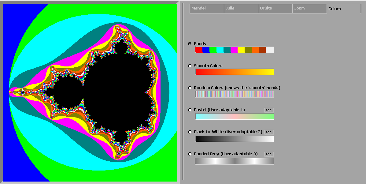
program will re-initialize itself, showing the default, banded Mandelbrot set. Smooth, grey-scale, zoomed-in: Colors-tab The Colors tab offers you a choice of 6 color gradations of
which 1 can be selected for use in the calculations. (Remember that the �Escape
Time (smooth)�-algorithm cannot use the first color-bar) -/Banded -/Red to Yellow -/Random -/Pastel -/Grayscale (Black to white) - Gives really nice results -/multiple grayscales Once your selection made, there is nothing left than to go
back to one of the other Tabs The last three color-bars however can be customized by the
user by pressing the small blue Set button. This will take you to a new Tab layout (but still under the
�Colors� label): The Color selector has a large RGB selector and an empty
color-bar. Slot 0 and Slot 255 have a special selector area to make selecting
start/end position easier. The usage scenario is as follows: select a color (eg red: 255,0,0) select Start position by clicking on the first white square under the colorbar. This will make a gradation from the chosen color to white select another color and click the End position by clicking on the second/rightmost white square under the colorbar. This will make a gradation from the first chosen color to the second You can now select a third, fourth.. color and click in the colorbar itself to have more color transitions Unfortunately, the color selection is a bit of a bad hack and things seem to break down if choosing too many colors�. Best keep it to three� Once done, you absolutely must press the OK- button in order to transfer the customized color-bar to the real color-bar. If, as is
want to happen, you make a mess of the colors, you can restart by clicking on the Cancel-button. Once done, you still need to select the radio-button next to your newly created color-bar before trying it out. Gallery Here are a few of the program�s outputs.